Comparando os Resultados da Estratégia de IFR2 nos Ativos do Ibovespa
O post de hoje é a continuação do artigo anterior, onde testamos a estratégia de IFR2 nos papeis mais fortes do Ibovespa, em uma janela de 100 dias, nos últimos 6 anos.
Nessa abordagem, a cada operação nós selecionávamos um novo ativo. Ao final, percebemos que um dos pontos fracos dessa estratégia é que acabávamos deixando de utilizar ativos que não apresentavam altas expressivas, mas que performariam bem no IFR2 (ex: EQTL3).
Para fins comparativos, no backtest de hoje nós testaremos a estratégia para todos os ativos que compõem a carteira do Ibovespa, no mesmo intervalo de tempo. Assim, poderemos ranquear os ativos de acordo com os melhores resultados e visualizar onde a estratégia anterior se encaixa.
Baixando os ativos que compõem a carteira do Ibovespa
Após baixar as bibliotecas necessárias, nós utilizaremos a mesma função get_ibov_tickers(), elaborada no último post.
OBS: Vamos remover ASAI3.SA da lista, uma vez que o ativo compõe o Ibovespa porém foi criado apenas em Março/2021.
# %%capture means we suppress the output
%%capture

import pandas as pd
import numpy as np
import matplotlib.pyplot as plt
!pip install yfinance
import yfinance as yf
def get_ibov_tickers():
url = "http://bvmf.bmfbovespa.com.br/indices/ResumoCarteiraTeorica.aspx?Indice=IBOV&idioma=pt-br"
html = pd.read_html(url, decimal=",", thousands=".", index_col="Código")[0][:-1]
tickers = (html.index + ".SA").to_list()
return tickers
tickers = get_ibov_tickers()
# Remove ticker without data
tickers.remove("ASAI3.SA")Faremos o download das colunas com o preço de abertura, fechamento e máxima, no mesmo intervalo de tempo (Janeiro/2015 - Dezembro/2020).
start = "2015-01-01"
end = "2020-12-30"
df = yf.download(tickers=tickers, start=start, end=end).copy()[["Open", "High", "Close"]]

df.head()
[*********************100%***********************] 81 of 81 completed
| Open | ... | Close | |||||||||||||||||||
|---|---|---|---|---|---|---|---|---|---|---|---|---|---|---|---|---|---|---|---|---|---|
| ABEV3.SA | AZUL4.SA | B3SA3.SA | BBAS3.SA | BBDC3.SA | BBDC4.SA | BBSE3.SA | BEEF3.SA | BPAC11.SA | BRAP4.SA | ... | TAEE11.SA | TIMS3.SA | TOTS3.SA | UGPA3.SA | USIM5.SA | VALE3.SA | VIVT3.SA | VVAR3.SA | WEGE3.SA | YDUQ3.SA | |
| Date | |||||||||||||||||||||
| 2015-01-02 | 16.139999 | NaN | 9.81 | 23.430000 | 15.969308 | 16.482443 | 31.850000 | 9.744451 | NaN | 14.06 | ... | 18.850000 | 11.74 | 11.910702 | 25.330000 | 4.79 | 21.280001 | 37.820000 | 6.80 | 11.846153 | 22.049999 |
| 2015-01-05 | 15.910000 | NaN | 9.43 | 22.580000 | 15.794703 | 15.989155 | 30.340000 | 9.301968 | NaN | 13.36 | ... | 18.780001 | 11.46 | 11.544731 | 24.655001 | 4.50 | 20.959999 | 37.070000 | 6.80 | 11.926923 | 20.730000 |
| 2015-01-06 | 15.730000 | NaN | 9.20 | 22.230000 | 16.021217 | 16.321175 | 29.450001 | 8.938149 | NaN | 13.51 | ... | 18.809999 | 11.44 | 10.822770 | 24.690001 | 4.72 | 21.799999 | 36.150002 | 6.80 | 11.750000 | 19.520000 |
| 2015-01-07 | 16.340000 | NaN | 9.40 | 22.940001 | 16.460091 | 17.046877 | 30.830000 | 8.800488 | NaN | 14.11 | ... | 18.840000 | 11.48 | 10.746248 | 25.360001 | 5.00 | 22.600000 | 37.389999 | 7.36 | 11.615384 | 18.910000 |
| 2015-01-08 | 16.430000 | NaN | 9.89 | 23.770000 | 16.993345 | 17.549650 | 30.590000 | 9.124975 | NaN | 14.67 | ... | 19.020000 | 12.00 | 10.995774 | 25.100000 | 4.75 | 22.840000 | 38.910000 | 7.36 | 11.811538 | 19.500000 |
5 rows × 243 columns
Também transformaremos a indexação em apenas um nível, para simplificar o acesso às colunas.
df.columns = [" ".join(col).strip() for col in df.columns.values]
df.head()| Open ABEV3.SA | Open AZUL4.SA | Open B3SA3.SA | Open BBAS3.SA | Open BBDC3.SA | Open BBDC4.SA | Open BBSE3.SA | Open BEEF3.SA | Open BPAC11.SA | Open BRAP4.SA | ... | Close TAEE11.SA | Close TIMS3.SA | Close TOTS3.SA | Close UGPA3.SA | Close USIM5.SA | Close VALE3.SA | Close VIVT3.SA | Close VVAR3.SA | Close WEGE3.SA | Close YDUQ3.SA | |
|---|---|---|---|---|---|---|---|---|---|---|---|---|---|---|---|---|---|---|---|---|---|
| Date | |||||||||||||||||||||
| 2015-01-02 | 16.139999 | NaN | 9.81 | 23.430000 | 15.969308 | 16.482443 | 31.850000 | 9.744451 | NaN | 14.06 | ... | 18.850000 | 11.74 | 11.910702 | 25.330000 | 4.79 | 21.280001 | 37.820000 | 6.80 | 11.846153 | 22.049999 |
| 2015-01-05 | 15.910000 | NaN | 9.43 | 22.580000 | 15.794703 | 15.989155 | 30.340000 | 9.301968 | NaN | 13.36 | ... | 18.780001 | 11.46 | 11.544731 | 24.655001 | 4.50 | 20.959999 | 37.070000 | 6.80 | 11.926923 | 20.730000 |
| 2015-01-06 | 15.730000 | NaN | 9.20 | 22.230000 | 16.021217 | 16.321175 | 29.450001 | 8.938149 | NaN | 13.51 | ... | 18.809999 | 11.44 | 10.822770 | 24.690001 | 4.72 | 21.799999 | 36.150002 | 6.80 | 11.750000 | 19.520000 |
| 2015-01-07 | 16.340000 | NaN | 9.40 | 22.940001 | 16.460091 | 17.046877 | 30.830000 | 8.800488 | NaN | 14.11 | ... | 18.840000 | 11.48 | 10.746248 | 25.360001 | 5.00 | 22.600000 | 37.389999 | 7.36 | 11.615384 | 18.910000 |
| 2015-01-08 | 16.430000 | NaN | 9.89 | 23.770000 | 16.993345 | 17.549650 | 30.590000 | 9.124975 | NaN | 14.67 | ... | 19.020000 | 12.00 | 10.995774 | 25.100000 | 4.75 | 22.840000 | 38.910000 | 7.36 | 11.811538 | 19.500000 |
5 rows × 243 columns
Calculando o IFR2 e os pontos de entrada e saída para cada ativo
Como de praxe, utilizaremos a função rsi() para calcular os valores de IFR para 2 períodos e strategy_points() para calcular os preços de compra e venda da estratégia. Lembrando que utilizaremos a estratégia original, caracterizada por pontos de entrada em valores de IFR2 abaixo ou iguais a 30 e pontos de saída na máxima dos dois dias anteriores.
def rsi(data, column, window=2):

    #data = data.copy()

    # Establish gains and losses for each day
    data["Variation"] = data[column].diff()
    data = data[1:]
    data["Gain"] = np.where(data["Variation"] > 0, data["Variation"], 0)
    data["Loss"] = np.where(data["Variation"] < 0, data["Variation"], 0)

    # Calculate simple averages so we can initialize the classic averages
    simple_avg_gain = data["Gain"].rolling(window).mean()
    simple_avg_loss = data["Loss"].abs().rolling(window).mean()
    classic_avg_gain = simple_avg_gain.copy()
    classic_avg_loss = simple_avg_loss.copy()

    for i in range(window, len(classic_avg_gain)):
        classic_avg_gain[i] = (classic_avg_gain[i - 1] * (window - 1) + data["Gain"].iloc[i]) / window
        classic_avg_loss[i] = (classic_avg_loss[i - 1] * (window - 1) + data["Loss"].abs().iloc[i]) / window

    # Calculate the RSI
    RS = classic_avg_gain / classic_avg_loss
    RSI = 100 - (100 / (1 + RS))

    return RSI
def strategy_points(data, rsi_parameter_entry=30):
data["Target1"] = data["High"].shift(1)
data["Target2"] = data["High"].shift(2)
data["Target"] = data[["Target1", "Target2"]].max(axis=1)
# We don't need them anymore
data.drop(columns=["Target1", "Target2"], inplace=True)
# Define exact buy price
data["Buy Price"] = np.where(data["IFR2"] <= rsi_parameter_entry, data["Close"], np.nan)
# Define exact sell price
data["Sell Price"] = np.where(
data["High"] > data['Target'],
np.where(data['Open'] > data['Target'], data['Open'], data['Target']),
np.nan)
return data Assim como foi feito no artigo anterior, vamos isolar as colunas de cada ativo em dataframes, armazenando-os no dicionário dict_of_df, através do loop abaixo. Desse modo, cada ativo (representando as chaves) terá seu próprio dataframe (representando os valores correspondentes).
Antes de utilizarmos as funções acima, temos que excluir valores NaN a fim de evitar possíveis erros em nossos códigos mais para frente. Faremos isso através da função .dropna().
dict_of_df = {}

for ticker in tickers:
    # Isolate the columns (open, high, close) of each asset into a dataframe
    # and store it in a dictionary 'dict_of_df'
    data = df[
        [("Open " + ticker),
         ("High " + ticker),
         ("Close " + ticker)]].copy()

    # Rename the columns
    data.rename(columns={
        ("Open " + ticker): 'Open',
        ("High " + ticker): 'High',
        ("Close " + ticker): 'Close'}, inplace=True)

    data.dropna(inplace=True)

    # Calculate IFR2 and add it to a new column
    data["IFR2"] = rsi(data=data, column="Close")

    # Calculate purchase and sale prices
    data = strategy_points(data)

    dict_of_df[ticker] = data
Realizando o backtest
Utilizaremos a estratégia com um stop de 7 dias, uma vez que esta foi a que apresentou melhores resultados no último backtest.
As funções a seguir foram desenvolvidas ao longo dessa série de artigos. Se você ainda não as conhece, não deixe de conferir os posts anteriores!
import math

# Create a function to round any number to the smalles multiple of 100
def round_down(x):
    return int(math.floor(x / 100.0)) * 100

def algorithm_with_stop(data, max_days, initial_capital=10000):

    # List with the total capital after every operation
    total_capital = [initial_capital]

    # List with profits for every operation. We initialize with 0 so
    # both lists have the same size
    all_profits = [0]

    days_in_operation = 0

    ongoing = False

    for i in range(0,len(data)):

        if ongoing == True:

            days_in_operation += 1

            # If any of the following conditions are met, the operation will end
            if days_in_operation == max_days or ~(np.isnan(data['Sell Price'][i])):

                # Define exit point and total profit
                exit = np.where(
                    ~(np.isnan(data['Sell Price'][i])),
                    data['Sell Price'][i],
                    data['Close'][i])

                profit = shares * (exit - entry)

                # Append profit to list and create a new entry with the capital
                # after the operation is complete
                all_profits += [profit]
                current_capital = total_capital[-1]
                total_capital += [current_capital + profit]

                ongoing = False

        else:
            if ~(np.isnan(data['Buy Price'][i])):
                entry = data['Buy Price'][i]
                shares = round_down(initial_capital / entry)
                days_in_operation = 0
                ongoing = True

    return all_profits, total_capital
def get_drawdown(data, column = "Close"):
data["Max"] = data[column].cummax()
data["Delta"] = data['Max'] - data[column]
data["Drawdown"] = 100 * (data["Delta"] / data["Max"])
max_drawdown = data["Drawdown"].max()
return max_drawdowndef strategy_test(all_profits, total_capital):
num_operations = (len(all_profits) - 1)
gains = sum(x >= 0 for x in all_profits)
pct_gains = 100 * (gains / num_operations)
losses = num_operations - gains
pct_losses = 100 - pct_gains
total_profit = sum(all_profits)
pct_profit = (total_profit / total_capital[0]) * 100
# Compute drawdown
total_capital = pd.DataFrame(data=total_capital, columns=["total_capital"])
drawdown = get_drawdown(data=total_capital, column="total_capital")
profit_per_operation = pct_profit / num_operations
return {
"num_operations": num_operations,
"gains": gains ,
"pct_gains": pct_gains.round(),
"losses": losses,
"pct_losses": pct_losses.round(),
"total_profit": total_profit,
"pct_profit": pct_profit,
"profit_per_operation": profit_per_operation,
"drawdown": drawdown
}Como o objetivo é realizar o backtest para cada ativo do Ibovespa, iteraremos sobre a lista de tickers, afim de utilizar as funções que rodam o algoritmo (algorithm_with_stop) e a estatítica (strategy_test) para cada um deles. Os resultados desta última serão armazenado no dicionário statistics.
statistics = {}

for ticker in tickers:
    data = dict_of_df[ticker]
    all_profits, total_capital = algorithm_with_stop(data=data, max_days=7)
    statistics[ticker] = strategy_test(all_profits, total_capital)
Vamos transformar statistics em um dataframe para uma melhor visualização dos dados.
statistics = pd.DataFrame.from_dict(statistics, orient="index").round(2)
statistics
| num_operations | gains | pct_gains | losses | pct_losses | total_profit | pct_profit | profit_per_operation | drawdown | |
|---|---|---|---|---|---|---|---|---|---|
| ABEV3.SA | 167 | 124 | 74.0 | 43 | 26.0 | 4899.00 | 48.99 | 0.29 | 26.27 |
| AZUL4.SA | 102 | 70 | 69.0 | 32 | 31.0 | 1869.00 | 18.69 | 0.18 | 52.24 |
| B3SA3.SA | 167 | 131 | 78.0 | 36 | 22.0 | 15232.00 | 152.32 | 0.91 | 11.07 |
| BBAS3.SA | 173 | 116 | 67.0 | 57 | 33.0 | 4111.00 | 41.11 | 0.24 | 28.28 |
| BBDC3.SA | 166 | 109 | 66.0 | 57 | 34.0 | 39.75 | 0.40 | 0.00 | 39.73 |
| ... | ... | ... | ... | ... | ... | ... | ... | ... | ... |
| VALE3.SA | 162 | 107 | 66.0 | 55 | 34.0 | 7176.00 | 71.76 | 0.44 | 62.17 |
| VIVT3.SA | 184 | 139 | 76.0 | 45 | 24.0 | 14010.00 | 140.10 | 0.76 | 16.21 |
| VVAR3.SA | 154 | 101 | 66.0 | 53 | 34.0 | 8767.00 | 87.67 | 0.57 | 68.31 |
| WEGE3.SA | 164 | 121 | 74.0 | 43 | 26.0 | 11089.16 | 110.89 | 0.68 | 15.44 |
| YDUQ3.SA | 167 | 114 | 68.0 | 53 | 32.0 | 5165.01 | 51.65 | 0.31 | 55.73 |
81 rows × 9 columns
Agora já podemos incluir a estatística da estratégia do último artigo nessa mesma tabela. Iremos chamá-la de IBOV Portfolio Strategy.
# Values were generated by running a prior backtest
statistics.loc["IBOV Portfolio Strategy"] = [72, 52, 72.0, 20, 28.0, 5842.15, 58.42, 0.81, 26.2]
statistics.tail()| num_operations | gains | pct_gains | losses | pct_losses | total_profit | pct_profit | profit_per_operation | drawdown | |
|---|---|---|---|---|---|---|---|---|---|
| VIVT3.SA | 184.0 | 139.0 | 76.0 | 45.0 | 24.0 | 14010.00 | 140.10 | 0.76 | 16.21 |
| VVAR3.SA | 154.0 | 101.0 | 66.0 | 53.0 | 34.0 | 8767.00 | 87.67 | 0.57 | 68.31 |
| WEGE3.SA | 164.0 | 121.0 | 74.0 | 43.0 | 26.0 | 11089.16 | 110.89 | 0.68 | 15.44 |
| YDUQ3.SA | 167.0 | 114.0 | 68.0 | 53.0 | 32.0 | 5165.01 | 51.65 | 0.31 | 55.73 |
| IBOV Portfolio Strategy | 72.0 | 52.0 | 72.0 | 20.0 | 28.0 | 5842.15 | 58.42 | 0.81 | 26.20 |
Plotando as informações mais relevantes
Uma vez que já temos o backtest para todos os ativos, vamos plotar o lucro por operação e o drawdown. Para isso, vamos primeiro ordenar nosso dataframe de acordo com essas colunas e separá-los em tabelas diferentes.
Faremos isso através da função .sort_values() do pandas, que recebe como argumento a coluna com os valores no qual se deseja ordenar o dataframe inteiro. Ao final, teremos uma tabela ordenada pelo lucro por operação (sorted_by_profit_per_operation) e outra pelo drawdown (sorted_by_drawdown).
A função pd.set_option() nos permite alterar o máximo de linhas a serem exibidas.
sorted_by_profit_per_operation = statistics.sort_values("profit_per_operation", ascending=False)
pd.set_option("display.max_rows", 100)
sorted_by_profit_per_operation
| num_operations | gains | pct_gains | losses | pct_losses | total_profit | pct_profit | profit_per_operation | drawdown | |
|---|---|---|---|---|---|---|---|---|---|
| PCAR3.SA | 104.0 | 89.0 | 86.0 | 15.0 | 14.0 | 15244.00 | 152.44 | 1.47 | 33.19 |
| NTCO3.SA | 31.0 | 24.0 | 77.0 | 7.0 | 23.0 | 4434.47 | 44.34 | 1.43 | 25.43 |
| LCAM3.SA | 158.0 | 121.0 | 77.0 | 37.0 | 23.0 | 18439.99 | 184.40 | 1.17 | 20.66 |
| ENGI11.SA | 154.0 | 122.0 | 79.0 | 32.0 | 21.0 | 14843.48 | 148.43 | 0.96 | 6.86 |
| TOTS3.SA | 173.0 | 131.0 | 76.0 | 42.0 | 24.0 | 16145.82 | 161.46 | 0.93 | 17.03 |
| B3SA3.SA | 167.0 | 131.0 | 78.0 | 36.0 | 22.0 | 15232.00 | 152.32 | 0.91 | 11.07 |
| EQTL3.SA | 168.0 | 126.0 | 75.0 | 42.0 | 25.0 | 15238.00 | 152.38 | 0.91 | 9.34 |
| CPLE6.SA | 177.0 | 129.0 | 73.0 | 48.0 | 27.0 | 16035.00 | 160.35 | 0.91 | 26.36 |
| LREN3.SA | 167.0 | 123.0 | 74.0 | 44.0 | 26.0 | 13965.04 | 139.65 | 0.84 | 11.48 |
| IBOV Portfolio Strategy | 72.0 | 52.0 | 72.0 | 20.0 | 28.0 | 5842.15 | 58.42 | 0.81 | 26.20 |
| FLRY3.SA | 171.0 | 129.0 | 75.0 | 42.0 | 25.0 | 13455.00 | 134.55 | 0.79 | 12.47 |
| VIVT3.SA | 184.0 | 139.0 | 76.0 | 45.0 | 24.0 | 14010.00 | 140.10 | 0.76 | 16.21 |
| SULA11.SA | 172.0 | 125.0 | 73.0 | 47.0 | 27.0 | 13128.92 | 131.29 | 0.76 | 14.78 |
| CRFB3.SA | 100.0 | 77.0 | 77.0 | 23.0 | 23.0 | 7641.00 | 76.41 | 0.76 | 10.65 |
| PRIO3.SA | 161.0 | 119.0 | 74.0 | 42.0 | 26.0 | 11902.10 | 119.02 | 0.74 | 38.29 |
| ENBR3.SA | 165.0 | 122.0 | 74.0 | 43.0 | 26.0 | 12107.73 | 121.08 | 0.73 | 11.01 |
| PETR3.SA | 160.0 | 108.0 | 68.0 | 52.0 | 32.0 | 11203.00 | 112.03 | 0.70 | 22.67 |
| RENT3.SA | 165.0 | 125.0 | 76.0 | 40.0 | 24.0 | 11538.69 | 115.39 | 0.70 | 22.12 |
| TIMS3.SA | 164.0 | 117.0 | 71.0 | 47.0 | 29.0 | 11319.99 | 113.20 | 0.69 | 11.46 |
| PETR4.SA | 157.0 | 106.0 | 68.0 | 51.0 | 32.0 | 10836.01 | 108.36 | 0.69 | 25.84 |
| WEGE3.SA | 164.0 | 121.0 | 74.0 | 43.0 | 26.0 | 11089.16 | 110.89 | 0.68 | 15.44 |
| CCRO3.SA | 180.0 | 125.0 | 69.0 | 55.0 | 31.0 | 12192.00 | 121.92 | 0.68 | 12.23 |
| MRVE3.SA | 165.0 | 118.0 | 72.0 | 47.0 | 28.0 | 11264.92 | 112.65 | 0.68 | 14.12 |
| JBSS3.SA | 171.0 | 128.0 | 75.0 | 43.0 | 25.0 | 11541.99 | 115.42 | 0.67 | 31.33 |
| MRFG3.SA | 183.0 | 134.0 | 73.0 | 49.0 | 27.0 | 12266.00 | 122.66 | 0.67 | 24.31 |
| CYRE3.SA | 175.0 | 129.0 | 74.0 | 46.0 | 26.0 | 11699.99 | 117.00 | 0.67 | 36.97 |
| SANB11.SA | 172.0 | 132.0 | 77.0 | 40.0 | 23.0 | 11216.00 | 112.16 | 0.65 | 12.35 |
| ENEV3.SA | 154.0 | 111.0 | 72.0 | 43.0 | 28.0 | 9901.32 | 99.01 | 0.64 | 36.18 |
| MULT3.SA | 173.0 | 129.0 | 75.0 | 44.0 | 25.0 | 10856.67 | 108.57 | 0.63 | 15.66 |
| RADL3.SA | 160.0 | 118.0 | 74.0 | 42.0 | 26.0 | 9945.40 | 99.45 | 0.62 | 11.44 |
| TAEE11.SA | 173.0 | 132.0 | 76.0 | 41.0 | 24.0 | 10732.00 | 107.32 | 0.62 | 7.09 |
| GNDI3.SA | 72.0 | 60.0 | 83.0 | 12.0 | 17.0 | 4376.09 | 43.76 | 0.61 | 21.21 |
| BRAP4.SA | 160.0 | 115.0 | 72.0 | 45.0 | 28.0 | 9444.00 | 94.44 | 0.59 | 70.12 |
| VVAR3.SA | 154.0 | 101.0 | 66.0 | 53.0 | 34.0 | 8767.00 | 87.67 | 0.57 | 68.31 |
| BPAC11.SA | 100.0 | 70.0 | 70.0 | 30.0 | 30.0 | 5397.00 | 53.97 | 0.54 | 27.71 |
| ECOR3.SA | 172.0 | 116.0 | 67.0 | 56.0 | 33.0 | 8557.00 | 85.57 | 0.50 | 34.92 |
| EGIE3.SA | 174.0 | 128.0 | 74.0 | 46.0 | 26.0 | 8487.80 | 84.88 | 0.49 | 6.82 |
| VALE3.SA | 162.0 | 107.0 | 66.0 | 55.0 | 34.0 | 7176.00 | 71.76 | 0.44 | 62.17 |
| HAPV3.SA | 67.0 | 45.0 | 67.0 | 22.0 | 33.0 | 2928.60 | 29.29 | 0.44 | 18.57 |
| EZTC3.SA | 162.0 | 115.0 | 71.0 | 47.0 | 29.0 | 7136.74 | 71.37 | 0.44 | 28.52 |
| BBSE3.SA | 175.0 | 117.0 | 67.0 | 58.0 | 33.0 | 7238.00 | 72.38 | 0.41 | 17.42 |
| CPFE3.SA | 156.0 | 117.0 | 75.0 | 39.0 | 25.0 | 6024.02 | 60.24 | 0.39 | 26.44 |
| LAME4.SA | 164.0 | 113.0 | 69.0 | 51.0 | 31.0 | 6449.92 | 64.50 | 0.39 | 28.49 |
| BRML3.SA | 175.0 | 124.0 | 71.0 | 51.0 | 29.0 | 6571.81 | 65.72 | 0.38 | 25.24 |
| BTOW3.SA | 165.0 | 103.0 | 62.0 | 62.0 | 38.0 | 5706.09 | 57.06 | 0.35 | 50.66 |
| ITUB4.SA | 172.0 | 120.0 | 70.0 | 52.0 | 30.0 | 5863.31 | 58.63 | 0.34 | 16.88 |
| YDUQ3.SA | 167.0 | 114.0 | 68.0 | 53.0 | 32.0 | 5165.01 | 51.65 | 0.31 | 55.73 |
| CMIG4.SA | 177.0 | 118.0 | 67.0 | 59.0 | 33.0 | 5508.20 | 55.08 | 0.31 | 47.85 |
| ELET3.SA | 171.0 | 113.0 | 66.0 | 58.0 | 34.0 | 5304.22 | 53.04 | 0.31 | 34.27 |
| BBDC4.SA | 167.0 | 112.0 | 67.0 | 55.0 | 33.0 | 4875.76 | 48.76 | 0.29 | 19.99 |
| SBSP3.SA | 157.0 | 109.0 | 69.0 | 48.0 | 31.0 | 4586.00 | 45.86 | 0.29 | 21.94 |
| ABEV3.SA | 167.0 | 124.0 | 74.0 | 43.0 | 26.0 | 4899.00 | 48.99 | 0.29 | 26.27 |
| KLBN11.SA | 169.0 | 119.0 | 70.0 | 50.0 | 30.0 | 4853.00 | 48.53 | 0.29 | 20.51 |
| CSAN3.SA | 162.0 | 113.0 | 70.0 | 49.0 | 30.0 | 4492.00 | 44.92 | 0.28 | 24.38 |
| MGLU3.SA | 146.0 | 97.0 | 66.0 | 49.0 | 34.0 | 4077.40 | 40.77 | 0.28 | 110.56 |
| UGPA3.SA | 171.0 | 119.0 | 70.0 | 52.0 | 30.0 | 4600.49 | 46.00 | 0.27 | 31.53 |
| IGTA3.SA | 161.0 | 111.0 | 69.0 | 50.0 | 31.0 | 4420.00 | 44.20 | 0.27 | 24.66 |
| BBAS3.SA | 173.0 | 116.0 | 67.0 | 57.0 | 33.0 | 4111.00 | 41.11 | 0.24 | 28.28 |
| JHSF3.SA | 168.0 | 110.0 | 65.0 | 58.0 | 35.0 | 4011.00 | 40.11 | 0.24 | 34.64 |
| ITSA4.SA | 176.0 | 122.0 | 69.0 | 54.0 | 31.0 | 4233.63 | 42.34 | 0.24 | 24.24 |
| HYPE3.SA | 164.0 | 115.0 | 70.0 | 49.0 | 30.0 | 3675.00 | 36.75 | 0.22 | 28.21 |
| GGBR4.SA | 166.0 | 109.0 | 66.0 | 57.0 | 34.0 | 3557.00 | 35.57 | 0.21 | 47.41 |
| AZUL4.SA | 102.0 | 70.0 | 69.0 | 32.0 | 31.0 | 1869.00 | 18.69 | 0.18 | 52.24 |
| BRKM5.SA | 169.0 | 116.0 | 69.0 | 53.0 | 31.0 | 2787.00 | 27.87 | 0.16 | 40.24 |
| EMBR3.SA | 171.0 | 115.0 | 67.0 | 56.0 | 33.0 | 2070.01 | 20.70 | 0.12 | 31.46 |
| QUAL3.SA | 163.0 | 111.0 | 68.0 | 52.0 | 32.0 | 1773.00 | 17.73 | 0.11 | 47.47 |
| RAIL3.SA | 158.0 | 108.0 | 68.0 | 50.0 | 32.0 | 994.65 | 9.95 | 0.06 | 103.31 |
| ELET6.SA | 161.0 | 98.0 | 61.0 | 63.0 | 39.0 | 528.00 | 5.28 | 0.03 | 35.75 |
| BBDC3.SA | 166.0 | 109.0 | 66.0 | 57.0 | 34.0 | 39.75 | 0.40 | 0.00 | 39.73 |
| GOAU4.SA | 167.0 | 117.0 | 70.0 | 50.0 | 30.0 | 54.99 | 0.55 | 0.00 | 141.33 |
| BEEF3.SA | 168.0 | 111.0 | 66.0 | 57.0 | 34.0 | -261.94 | -2.62 | -0.02 | 50.04 |
| CVCB3.SA | 169.0 | 116.0 | 69.0 | 53.0 | 31.0 | -278.32 | -2.78 | -0.02 | 57.04 |
| CSNA3.SA | 161.0 | 100.0 | 62.0 | 61.0 | 38.0 | -703.00 | -7.03 | -0.04 | 80.61 |
| USIM5.SA | 159.0 | 106.0 | 67.0 | 53.0 | 33.0 | -794.00 | -7.94 | -0.05 | 99.44 |
| CIEL3.SA | 181.0 | 117.0 | 65.0 | 64.0 | 35.0 | -1530.71 | -15.31 | -0.08 | 75.26 |
| SUZB3.SA | 82.0 | 57.0 | 70.0 | 25.0 | 30.0 | -1084.00 | -10.84 | -0.13 | 43.75 |
| BRDT3.SA | 75.0 | 49.0 | 65.0 | 26.0 | 35.0 | -1424.00 | -14.24 | -0.19 | 38.78 |
| COGN3.SA | 170.0 | 104.0 | 61.0 | 66.0 | 39.0 | -3530.00 | -35.30 | -0.21 | 61.17 |
| HGTX3.SA | 93.0 | 58.0 | 62.0 | 35.0 | 38.0 | -2112.99 | -21.13 | -0.23 | 83.84 |
| BRFS3.SA | 169.0 | 106.0 | 63.0 | 63.0 | 37.0 | -4649.99 | -46.50 | -0.28 | 74.57 |
| GOLL4.SA | 170.0 | 112.0 | 66.0 | 58.0 | 34.0 | -5540.00 | -55.40 | -0.33 | 135.63 |
| IRBR3.SA | 93.0 | 67.0 | 72.0 | 26.0 | 28.0 | -4434.52 | -44.35 | -0.48 | 79.71 |
sorted_by_drawdown = statistics.sort_values("drawdown")
pd.set_option("display.max_rows", 100)
sorted_by_drawdown
| num_operations | gains | pct_gains | losses | pct_losses | total_profit | pct_profit | profit_per_operation | drawdown | |
|---|---|---|---|---|---|---|---|---|---|
| EGIE3.SA | 174.0 | 128.0 | 74.0 | 46.0 | 26.0 | 8487.80 | 84.88 | 0.49 | 6.82 |
| ENGI11.SA | 154.0 | 122.0 | 79.0 | 32.0 | 21.0 | 14843.48 | 148.43 | 0.96 | 6.86 |
| TAEE11.SA | 173.0 | 132.0 | 76.0 | 41.0 | 24.0 | 10732.00 | 107.32 | 0.62 | 7.09 |
| EQTL3.SA | 168.0 | 126.0 | 75.0 | 42.0 | 25.0 | 15238.00 | 152.38 | 0.91 | 9.34 |
| CRFB3.SA | 100.0 | 77.0 | 77.0 | 23.0 | 23.0 | 7641.00 | 76.41 | 0.76 | 10.65 |
| ENBR3.SA | 165.0 | 122.0 | 74.0 | 43.0 | 26.0 | 12107.73 | 121.08 | 0.73 | 11.01 |
| B3SA3.SA | 167.0 | 131.0 | 78.0 | 36.0 | 22.0 | 15232.00 | 152.32 | 0.91 | 11.07 |
| RADL3.SA | 160.0 | 118.0 | 74.0 | 42.0 | 26.0 | 9945.40 | 99.45 | 0.62 | 11.44 |
| TIMS3.SA | 164.0 | 117.0 | 71.0 | 47.0 | 29.0 | 11319.99 | 113.20 | 0.69 | 11.46 |
| LREN3.SA | 167.0 | 123.0 | 74.0 | 44.0 | 26.0 | 13965.04 | 139.65 | 0.84 | 11.48 |
| CCRO3.SA | 180.0 | 125.0 | 69.0 | 55.0 | 31.0 | 12192.00 | 121.92 | 0.68 | 12.23 |
| SANB11.SA | 172.0 | 132.0 | 77.0 | 40.0 | 23.0 | 11216.00 | 112.16 | 0.65 | 12.35 |
| FLRY3.SA | 171.0 | 129.0 | 75.0 | 42.0 | 25.0 | 13455.00 | 134.55 | 0.79 | 12.47 |
| MRVE3.SA | 165.0 | 118.0 | 72.0 | 47.0 | 28.0 | 11264.92 | 112.65 | 0.68 | 14.12 |
| SULA11.SA | 172.0 | 125.0 | 73.0 | 47.0 | 27.0 | 13128.92 | 131.29 | 0.76 | 14.78 |
| WEGE3.SA | 164.0 | 121.0 | 74.0 | 43.0 | 26.0 | 11089.16 | 110.89 | 0.68 | 15.44 |
| MULT3.SA | 173.0 | 129.0 | 75.0 | 44.0 | 25.0 | 10856.67 | 108.57 | 0.63 | 15.66 |
| VIVT3.SA | 184.0 | 139.0 | 76.0 | 45.0 | 24.0 | 14010.00 | 140.10 | 0.76 | 16.21 |
| ITUB4.SA | 172.0 | 120.0 | 70.0 | 52.0 | 30.0 | 5863.31 | 58.63 | 0.34 | 16.88 |
| TOTS3.SA | 173.0 | 131.0 | 76.0 | 42.0 | 24.0 | 16145.82 | 161.46 | 0.93 | 17.03 |
| BBSE3.SA | 175.0 | 117.0 | 67.0 | 58.0 | 33.0 | 7238.00 | 72.38 | 0.41 | 17.42 |
| HAPV3.SA | 67.0 | 45.0 | 67.0 | 22.0 | 33.0 | 2928.60 | 29.29 | 0.44 | 18.57 |
| BBDC4.SA | 167.0 | 112.0 | 67.0 | 55.0 | 33.0 | 4875.76 | 48.76 | 0.29 | 19.99 |
| KLBN11.SA | 169.0 | 119.0 | 70.0 | 50.0 | 30.0 | 4853.00 | 48.53 | 0.29 | 20.51 |
| LCAM3.SA | 158.0 | 121.0 | 77.0 | 37.0 | 23.0 | 18439.99 | 184.40 | 1.17 | 20.66 |
| GNDI3.SA | 72.0 | 60.0 | 83.0 | 12.0 | 17.0 | 4376.09 | 43.76 | 0.61 | 21.21 |
| SBSP3.SA | 157.0 | 109.0 | 69.0 | 48.0 | 31.0 | 4586.00 | 45.86 | 0.29 | 21.94 |
| RENT3.SA | 165.0 | 125.0 | 76.0 | 40.0 | 24.0 | 11538.69 | 115.39 | 0.70 | 22.12 |
| PETR3.SA | 160.0 | 108.0 | 68.0 | 52.0 | 32.0 | 11203.00 | 112.03 | 0.70 | 22.67 |
| ITSA4.SA | 176.0 | 122.0 | 69.0 | 54.0 | 31.0 | 4233.63 | 42.34 | 0.24 | 24.24 |
| MRFG3.SA | 183.0 | 134.0 | 73.0 | 49.0 | 27.0 | 12266.00 | 122.66 | 0.67 | 24.31 |
| CSAN3.SA | 162.0 | 113.0 | 70.0 | 49.0 | 30.0 | 4492.00 | 44.92 | 0.28 | 24.38 |
| IGTA3.SA | 161.0 | 111.0 | 69.0 | 50.0 | 31.0 | 4420.00 | 44.20 | 0.27 | 24.66 |
| BRML3.SA | 175.0 | 124.0 | 71.0 | 51.0 | 29.0 | 6571.81 | 65.72 | 0.38 | 25.24 |
| NTCO3.SA | 31.0 | 24.0 | 77.0 | 7.0 | 23.0 | 4434.47 | 44.34 | 1.43 | 25.43 |
| PETR4.SA | 157.0 | 106.0 | 68.0 | 51.0 | 32.0 | 10836.01 | 108.36 | 0.69 | 25.84 |
| IBOV Portfolio Strategy | 72.0 | 52.0 | 72.0 | 20.0 | 28.0 | 5842.15 | 58.42 | 0.81 | 26.20 |
| ABEV3.SA | 167.0 | 124.0 | 74.0 | 43.0 | 26.0 | 4899.00 | 48.99 | 0.29 | 26.27 |
| CPLE6.SA | 177.0 | 129.0 | 73.0 | 48.0 | 27.0 | 16035.00 | 160.35 | 0.91 | 26.36 |
| CPFE3.SA | 156.0 | 117.0 | 75.0 | 39.0 | 25.0 | 6024.02 | 60.24 | 0.39 | 26.44 |
| BPAC11.SA | 100.0 | 70.0 | 70.0 | 30.0 | 30.0 | 5397.00 | 53.97 | 0.54 | 27.71 |
| HYPE3.SA | 164.0 | 115.0 | 70.0 | 49.0 | 30.0 | 3675.00 | 36.75 | 0.22 | 28.21 |
| BBAS3.SA | 173.0 | 116.0 | 67.0 | 57.0 | 33.0 | 4111.00 | 41.11 | 0.24 | 28.28 |
| LAME4.SA | 164.0 | 113.0 | 69.0 | 51.0 | 31.0 | 6449.92 | 64.50 | 0.39 | 28.49 |
| EZTC3.SA | 162.0 | 115.0 | 71.0 | 47.0 | 29.0 | 7136.74 | 71.37 | 0.44 | 28.52 |
| JBSS3.SA | 171.0 | 128.0 | 75.0 | 43.0 | 25.0 | 11541.99 | 115.42 | 0.67 | 31.33 |
| EMBR3.SA | 171.0 | 115.0 | 67.0 | 56.0 | 33.0 | 2070.01 | 20.70 | 0.12 | 31.46 |
| UGPA3.SA | 171.0 | 119.0 | 70.0 | 52.0 | 30.0 | 4600.49 | 46.00 | 0.27 | 31.53 |
| PCAR3.SA | 104.0 | 89.0 | 86.0 | 15.0 | 14.0 | 15244.00 | 152.44 | 1.47 | 33.19 |
| ELET3.SA | 171.0 | 113.0 | 66.0 | 58.0 | 34.0 | 5304.22 | 53.04 | 0.31 | 34.27 |
| JHSF3.SA | 168.0 | 110.0 | 65.0 | 58.0 | 35.0 | 4011.00 | 40.11 | 0.24 | 34.64 |
| ECOR3.SA | 172.0 | 116.0 | 67.0 | 56.0 | 33.0 | 8557.00 | 85.57 | 0.50 | 34.92 |
| ELET6.SA | 161.0 | 98.0 | 61.0 | 63.0 | 39.0 | 528.00 | 5.28 | 0.03 | 35.75 |
| ENEV3.SA | 154.0 | 111.0 | 72.0 | 43.0 | 28.0 | 9901.32 | 99.01 | 0.64 | 36.18 |
| CYRE3.SA | 175.0 | 129.0 | 74.0 | 46.0 | 26.0 | 11699.99 | 117.00 | 0.67 | 36.97 |
| PRIO3.SA | 161.0 | 119.0 | 74.0 | 42.0 | 26.0 | 11902.10 | 119.02 | 0.74 | 38.29 |
| BRDT3.SA | 75.0 | 49.0 | 65.0 | 26.0 | 35.0 | -1424.00 | -14.24 | -0.19 | 38.78 |
| BBDC3.SA | 166.0 | 109.0 | 66.0 | 57.0 | 34.0 | 39.75 | 0.40 | 0.00 | 39.73 |
| BRKM5.SA | 169.0 | 116.0 | 69.0 | 53.0 | 31.0 | 2787.00 | 27.87 | 0.16 | 40.24 |
| SUZB3.SA | 82.0 | 57.0 | 70.0 | 25.0 | 30.0 | -1084.00 | -10.84 | -0.13 | 43.75 |
| GGBR4.SA | 166.0 | 109.0 | 66.0 | 57.0 | 34.0 | 3557.00 | 35.57 | 0.21 | 47.41 |
| QUAL3.SA | 163.0 | 111.0 | 68.0 | 52.0 | 32.0 | 1773.00 | 17.73 | 0.11 | 47.47 |
| CMIG4.SA | 177.0 | 118.0 | 67.0 | 59.0 | 33.0 | 5508.20 | 55.08 | 0.31 | 47.85 |
| BEEF3.SA | 168.0 | 111.0 | 66.0 | 57.0 | 34.0 | -261.94 | -2.62 | -0.02 | 50.04 |
| BTOW3.SA | 165.0 | 103.0 | 62.0 | 62.0 | 38.0 | 5706.09 | 57.06 | 0.35 | 50.66 |
| AZUL4.SA | 102.0 | 70.0 | 69.0 | 32.0 | 31.0 | 1869.00 | 18.69 | 0.18 | 52.24 |
| YDUQ3.SA | 167.0 | 114.0 | 68.0 | 53.0 | 32.0 | 5165.01 | 51.65 | 0.31 | 55.73 |
| CVCB3.SA | 169.0 | 116.0 | 69.0 | 53.0 | 31.0 | -278.32 | -2.78 | -0.02 | 57.04 |
| COGN3.SA | 170.0 | 104.0 | 61.0 | 66.0 | 39.0 | -3530.00 | -35.30 | -0.21 | 61.17 |
| VALE3.SA | 162.0 | 107.0 | 66.0 | 55.0 | 34.0 | 7176.00 | 71.76 | 0.44 | 62.17 |
| VVAR3.SA | 154.0 | 101.0 | 66.0 | 53.0 | 34.0 | 8767.00 | 87.67 | 0.57 | 68.31 |
| BRAP4.SA | 160.0 | 115.0 | 72.0 | 45.0 | 28.0 | 9444.00 | 94.44 | 0.59 | 70.12 |
| BRFS3.SA | 169.0 | 106.0 | 63.0 | 63.0 | 37.0 | -4649.99 | -46.50 | -0.28 | 74.57 |
| CIEL3.SA | 181.0 | 117.0 | 65.0 | 64.0 | 35.0 | -1530.71 | -15.31 | -0.08 | 75.26 |
| IRBR3.SA | 93.0 | 67.0 | 72.0 | 26.0 | 28.0 | -4434.52 | -44.35 | -0.48 | 79.71 |
| CSNA3.SA | 161.0 | 100.0 | 62.0 | 61.0 | 38.0 | -703.00 | -7.03 | -0.04 | 80.61 |
| HGTX3.SA | 93.0 | 58.0 | 62.0 | 35.0 | 38.0 | -2112.99 | -21.13 | -0.23 | 83.84 |
| USIM5.SA | 159.0 | 106.0 | 67.0 | 53.0 | 33.0 | -794.00 | -7.94 | -0.05 | 99.44 |
| RAIL3.SA | 158.0 | 108.0 | 68.0 | 50.0 | 32.0 | 994.65 | 9.95 | 0.06 | 103.31 |
| MGLU3.SA | 146.0 | 97.0 | 66.0 | 49.0 | 34.0 | 4077.40 | 40.77 | 0.28 | 110.56 |
| GOLL4.SA | 170.0 | 112.0 | 66.0 | 58.0 | 34.0 | -5540.00 | -55.40 | -0.33 | 135.63 |
| GOAU4.SA | 167.0 | 117.0 | 70.0 | 50.0 | 30.0 | 54.99 | 0.55 | 0.00 | 141.33 |
OBS: Repare que nós temos drawdowns acima de 100%. Isso ocorre pois a estratégia sempre investe uma quantia fixa de capital (initial_capital). Sendo assim, ativos que tiverem prejuízos acima do capital initial vão apresentar drawdown superior a 100%.
Por fim, criaremos uma função para plotar os gráficos em barras horizontais, plot_barh, que receberá os seguintes argumentos:
- os valores do eixo x (
x); - os valores do eixo y (
y); - a legenda do eixo x (
x_label); - o título (
title); - o tamanho do gráfico (
figsize), que terá como padrão (12, 18); - se existe um índice que deseja-se destacar (
highlights_index) que, por padrão, seráNone; - e
invert_yaxiscaso seja necessário inverter a ordem do eixo y. Sendo assim, ele será falso (False), por padrão.
def plot_barh(x, y, x_label, title, figsize=(12, 18), highlights_index=None, invert_yaxis=False):
    fig = plt.figure(figsize=figsize)

    positives = x > 0
    graph = plt.barh(y, x, color=positives.map({True: "#49ce8b", False: "r"}))

    if highlights_index != None:
        graph[y.get_loc(highlights_index)].set_color("#033660")

    plt.margins(y=0.01)
    plt.xlabel(x_label, fontsize='x-large')
    plt.title(title, fontsize='xx-large')

    if invert_yaxis == True:
        plt.gca().invert_yaxis()

    return graph
Vamos plotar primeiro todos os ativos de acordo com o lucro por operação para termos uma visualização geral do ranking de backtest. Além disso, vamos destacar a estratégia do backtest passado.
plot_barh(
    x=sorted_by_profit_per_operation["profit_per_operation"],
    y=sorted_by_profit_per_operation.index,
    x_label="Lucro por Operação (%)",
    title="Backtest da estratégia de IFR2 aplicada nos ativos do Ibovespa, nos últimos 6 anos",
    highlights_index="IBOV Portfolio Strategy"
)
<BarContainer object of 82 artists>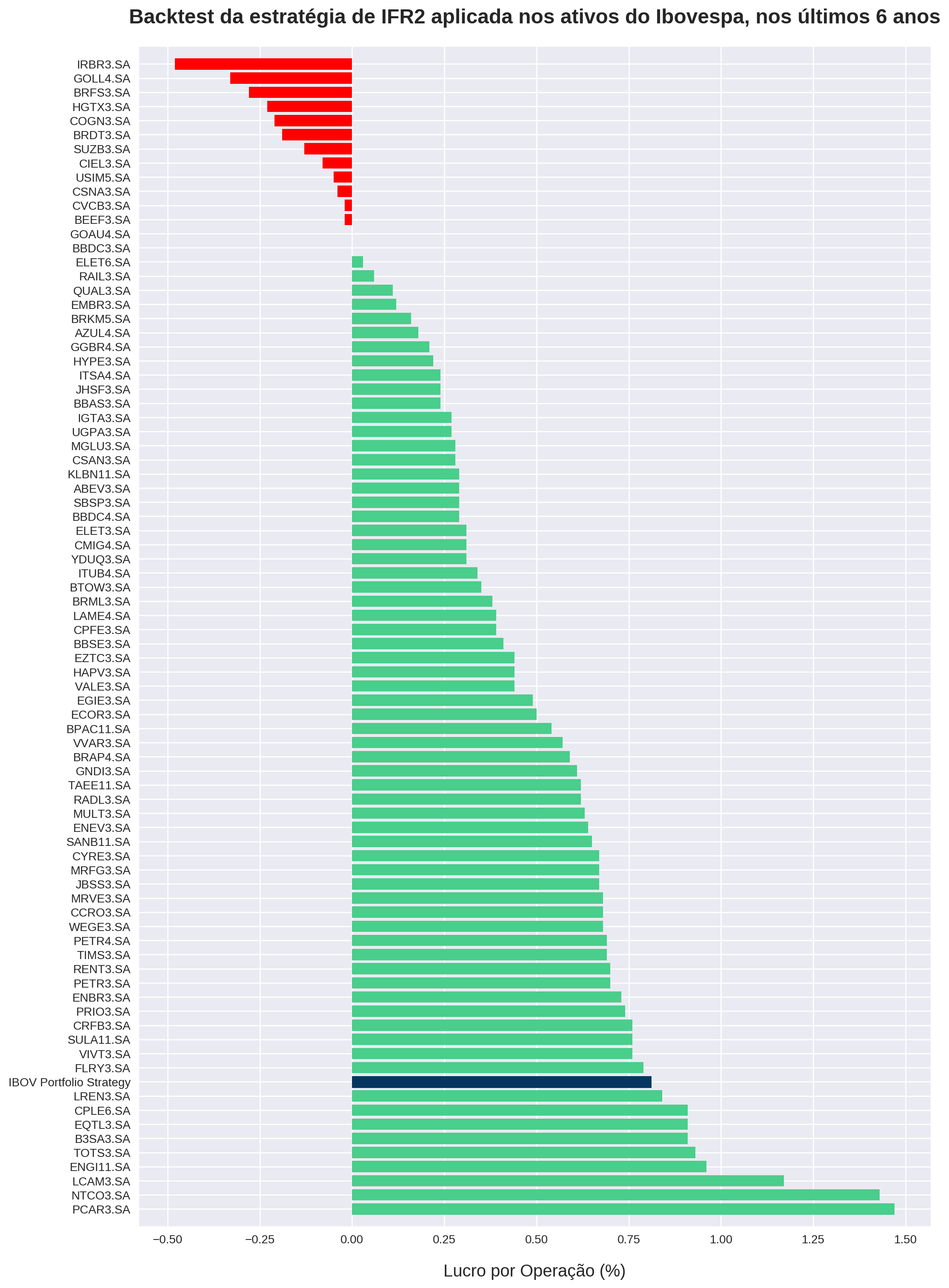
Agora vamos isolar os 10 melhores e os 10 piores resultados em relação ao lucro por operação.
top_10_profit_per_operation = sorted_by_profit_per_operation[:10]["profit_per_operation"]

plot_barh(
    x=top_10_profit_per_operation,
    y=top_10_profit_per_operation.index,
    x_label="Lucro por Operação (%)",
    title="Top 10 ativos do Ibovespa na estratégia de IFR2, nos últimos 6 anos",
    figsize=(8,6),
    highlights_index="IBOV Portfolio Strategy",
    invert_yaxis=True
)
<BarContainer object of 10 artists>
bottom_10_profit_per_operation = sorted_by_profit_per_operation[-10:]["profit_per_operation"]

plot_barh(
    x=bottom_10_profit_per_operation,
    y=bottom_10_profit_per_operation.index,
    x_label="Lucro por Operação (%)",
    title="Os 10 piores ativos do Ibovespa na estratégia de IFR2, nos últimos 6 anos",
    figsize=(8,6)
)
<BarContainer object of 10 artists>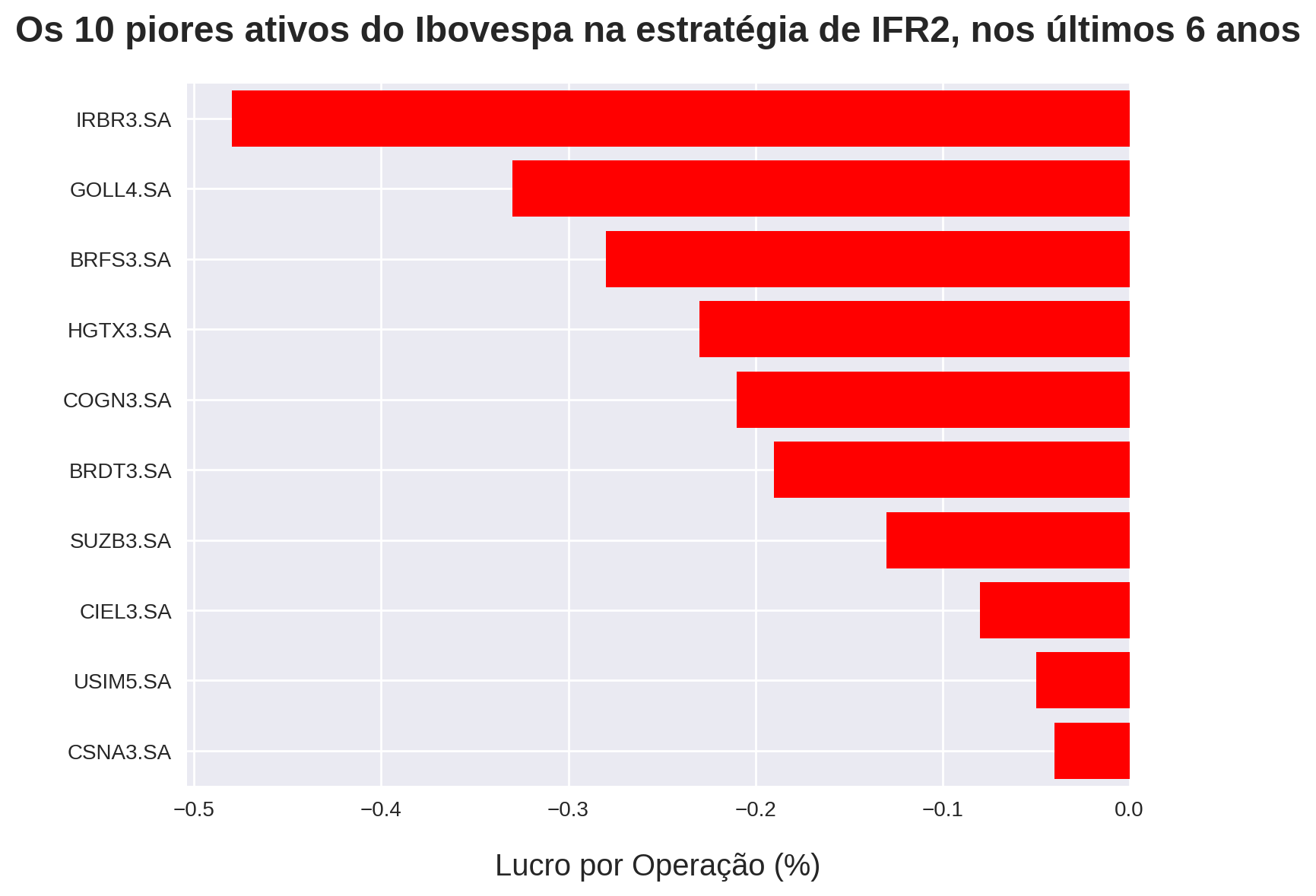
Vamos plotar também o top 10 no que diz respeito ao drawdown:
top_10_drawdown = sorted_by_drawdown[:10]["drawdown"]

plot_barh(
    x=top_10_drawdown,
    y=top_10_drawdown.index,
    x_label="Drawdown(%)",
    title="Top 10 ativos (do Ibovespa) com o melhor drawdown na estratégia de IFR2, nos últimos 6 anos",
    figsize=(10,6),
    invert_yaxis=True
)
<BarContainer object of 10 artists>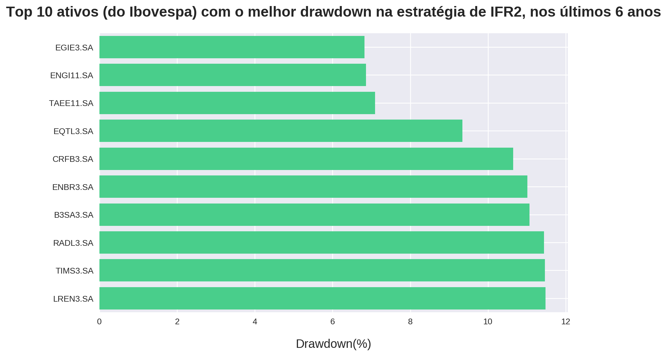
Por fim, vamos isolar os ativos em comum entre top_10_profit_per_operation e top_10_drawdown:
common = top_10_profit_per_operation[
    top_10_profit_per_operation.index.isin(
        top_10_drawdown.index
    )]

print(common)
ENGI11.SA 0.96
B3SA3.SA 0.91
EQTL3.SA 0.91
LREN3.SA 0.84
Name: profit_per_operation, dtype: float64
Conclusão
A tabela a seguir exibe os melhores ativos do IBOV em termos de Lucro / Operação e Drawdown:
| Lucro / Operação (%) | Drawdown (%) |
|---|---|
| PCAR3 | TIMS3 |
| NTCO3 | EGIE3 |
| LCAM3 | ENGI11 |
| ENGI11 | TAEE11 |
| TOTS3 | EQTL3 |
| EQTL3 | CRFB3 |
| CPLE6 | ENBR3 |
| B3SA3 | B3SA3 |
| LREN3 | RADL3 |
| IBOV Portfolio Strategy | LREN3 |
Observe que a estratégia utilizando a lista dinâmica está presente no top 10. Sendo assim, como discutimos no último artigo, esta se torna uma excelente alternativa para quem busca se proteger caso a estratégia de IFR2 pare de funcionar em um determinado ativo.
Como esperado, papeis que não figuraram na lista dos mais fortes do Ibovespa, como EQTL3 e LREN3, apresentaram um dos melhores resultados não só no lucro por operação, como também no drawdown. Já papeis que fizeram parte dessa lista, como GOLL4, HGTX3, SUZB3, USIM5 e CSNA3, demonstraram baixos lucros por operação.
Uma explicação para esse resultado está atrelada à volatilidade desses papeis. Para se sair bem na estratégia de IFR2, um ativo não precisa fazer fortes movimentações de alta, desde que oscile de forma previsível num range de preços.
Isso se confirma ao observarmos que metade dos ativos que tiveram os melhores resultados, principalmente em relação ao drawdown, correspondem a empresas do setor elétrico (EGIE3, TAEE11, ENGI11, EQTL3, ENBR3). Essas são empresas de rendimentos mais previsíveis e que distribuem dividendos, o que as tornam menos voláteis e, portanto, favoráveis à estratégia de IFR2.
Concluindo, no post de hoje nós criamos um ranking dos melhores resultados de backtests da estratégia de IFR2 nos últimos 6 anos. Você pode utilizá-lo juntamente com nossa nova ferramenta e otimizar seus resultados para essa estratégia!
Inscreva-se no canal do QuantBrasil!
Acompanhe novidades sobre a plataforma, vídeos sobre finanças quantitativas, tutoriais sobre programação e Inteligência Artificial!